
Why look at PD at scale?
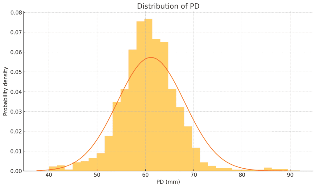
The average pupillary distance across 14,904 real-world Optogrid measurements is 61.2 mm (median 60.6 mm), with 90% of adults falling between 51.5 mm and 71.1 mm. These figures align with published clinical ranges and confirm that remote photo-based PD measurement captures the same population distribution as in-office instruments.
Pupillary distance (PD), the millimetres between the centres of your pupils, is the silent hero behind lens alignment. When PD is off, even a perfect prescription can feel blurry or induce strain. Because Optogrid captures PD remotely, we now have thousands of real-world readings instead of the handful an optician might see in a day. Analyzing them shows us interesting aspects of the human face and tells the truth without guesswork.
Our dataset in a nutshell
- Source: Every PD captured by Optogrid between January and June 2025.
- Sample size: 14904 unique sessions after scrubbing obviously invalid rows (see Methods note below).
- Fields: Single binocular PD plus dual PD for left and right eyes.
- Cleaning rules: Kept values in plausible adult ranges (40‑90 mm for single PD, 15‑50 mm per eye).
The bell curve in numbers
| Metric | Single PD |
|---|---|
| Mean | 61.2 mm |
| Median | 60.6 mm |
| Standard deviation | 7.0 mm |
| 5th–95th percentile | 51.5–71.1 mm |
| Maximum | 89.5 mm |
The histogram fits a textbook normal curve with one curiosity: a small “second hump” beyond 80 mm that accounts for just under 1 % of users. We will revisit that in a moment.
What This Dataset Does Not Show: Left-Right Symmetry
An earlier version of this post reported monocular averages of 30.54 mm (left) and 30.57 mm (right) and concluded that the two eyes stay in lock-step. That conclusion does not follow from that statistic. Averaging every left value and every right value separately cancels individual asymmetry: a patient at 33/29 mm and a patient at 29/33 mm pull the two means back together and contribute nothing to the gap between them. Asymmetry is described by the absolute difference per person, which this analysis never computed.
The agreement between the summed dual PD and the single binocular PD has the same problem. Where the binocular value is derived as the sum of the two monocular values, that agreement is arithmetic. It cannot tell you whether either number is correct.
For the actual shape of monocular asymmetry, published clinical data is the better source. In a 2021 study of 199 adults, mean monocular distance PD was 30.4 ± 1.7 mm on the right against 29.9 ± 1.5 mm on the left, and the right eye measured wider in 57% of participants (Gantz et al., Journal of Optometry, 2021). The population-average gap is roughly 0.5 mm and individual patients fall well outside it, which is why monocular PD is measured per eye rather than split from a binocular total.
How do our numbers compare to the literature?
Published sources cluster adult PD around the low 60s. Warby Parker cites a typical range of 60‑64 mm, Zenni Optical gives 54‑74 mm, and the Cleveland Clinic pegs the average at 63 mm. (warbyparker.com, zennioptical.com, my.clevelandclinic.org) Our mean of 61 mm and 5th‑to‑95th spread of 51‑71 mm fit snugly inside those brackets. In other words, our remote tool is mapping the same population curve traditional clinics see.
For a deeper look at how remote measurement stacks up against traditional PD rulers and digital lensmeter measurements, see our comparison of four PD measurement methods.
The story behind the high‑right tail
Why do 104 people register PDs of 80 mm or more?
- Big heads are real. Anthropometry studies put the tallest 2‑3 % of males above 78 mm.
- Scale drift. If the reference card tilts forward, its apparent width shrinks and every distance inflates by the same factor. Because dual PD tracks single PD precisely in this cluster, scale drift is a likely co‑conspirator.
We are adding a card‑angle check so future posts can separate biological giants from geometric artefacts.
Why it matters for online eyewear
- Lens accuracy: Sub-millimetre PD error keeps prism within ISO tolerances, reducing returns.
- Frame recommendations: Knowing that half the audience sits between 58‑64 mm lets us tailor which SKUs appear first.
- UX prompts: Only 1 in 60 users produce an extreme PD, so nudging just that slice to re‑capture keeps friction low for everyone else.
Accurate PD also directly affects other fitting parameters. Our guide on segment height for progressive lenses explains how PD and fitting height interact when dispensing multifocals. It is also worth noting that our dataset covers adults; pediatric PDs are notably smaller and age-dependent. If you fit children, see our dedicated resource on measuring PD in children for age-stratified reference ranges.
What’s next
Our next data drop will cross‑reference PD with self‑reported country to see if regional genetics show up. We will also slice by other dimensions. Male users have on average higher PD measurements, but for privacy reasons, we can’t tag that information in the measurement data.
If you want to start capturing your own patient PD data remotely, try Optogrid. Measurements take under two minutes with a smartphone and a standard reference card, and our step-by-step PD measurement guide walks through the process. You can also set up custom references to improve scale accuracy across different card types.
Methods note
Full cleaning and analysis recipe (Python + pandas). It loads the CSV, coerces numeric types, applies range filters, and overlays a normal probability density on a 30‑bin histogram.
import pandas as pd
import numpy as np
import matplotlib.pyplot as plt
from ace_tools import display_dataframe_to_user

# 1. Load the raw file
df = pd.read_csv('./optogrid_production_20250630_171750.csv',
                 header=None,
                 names=['PD', 'PD_L', 'PD_R'])

# 2. Convert to numeric and drop obviously invalid (non‑numeric / NaNs / ±inf)
df = df.apply(pd.to_numeric, errors='coerce')
df = df.replace([np.inf, -np.inf], np.nan).dropna()

# 3. Simple physiological range filter to cull extreme outliers
outlier_mask = (
    (df['PD'] < 40) | (df['PD'] > 90) |   # monocular PD usually 50‑75 mm
    (df['PD_L'] < 15) | (df['PD_L'] > 50) |
    (df['PD_R'] < 15) | (df['PD_R'] > 50)
)
df_final = df[~outlier_mask].copy()

# 4. Extra derived columns for deeper inspection
df_final['PD_sumLR'] = df_final['PD_L'] + df_final['PD_R']
df_final['PD_diff'] = df_final['PD'] - df_final['PD_sumLR']

# 5. Descriptive statistics table
summary = df_final[['PD', 'PD_L', 'PD_R', 'PD_diff']].describe().T.round(2)
display_dataframe_to_user("Cleaned PD Summary", summary)

# 6. Bell‑curve style histograms with overlaid normal PDF
for column in ['PD', 'PD_L', 'PD_R']:
    data = df_final[column]
    mean = data.mean()
    std = data.std()

    plt.figure()
    plt.hist(data, bins=30, density=True, alpha=0.6)

    # overlay the theoretical normal curve
    xmin, xmax = plt.xlim()
    x = np.linspace(xmin, xmax, 400)
    pdf = (1 / (std * np.sqrt(2 * np.pi))) * np.exp(-((x - mean) ** 2) / (2 * std ** 2))
    plt.plot(x, pdf)

    plt.title(f"Distribution of {column}")
    plt.xlabel(f"{column} (mm)")
    plt.ylabel("Probability density")
    plt.tight_layout()
    plt.show()
I grew up inside an optical shop. My mother likes to tell how, as a kid, I would watch eyeglasses being assembled, play with the tools, and draw on the back of service order slips. The family business taught me early what a precise measurement and work done right are worth.
I went on to spend more than twenty years as a software engineer, always keeping an eye on the optical world. Optogrid was born where the two meet: digital measurement technology (pupillary distance and fitting heights) built by someone who knows the dispensing counter from the inside.